Machine Learning Predictions of GDP at higher spatial and sectoral resolution
Preprint on SSRN
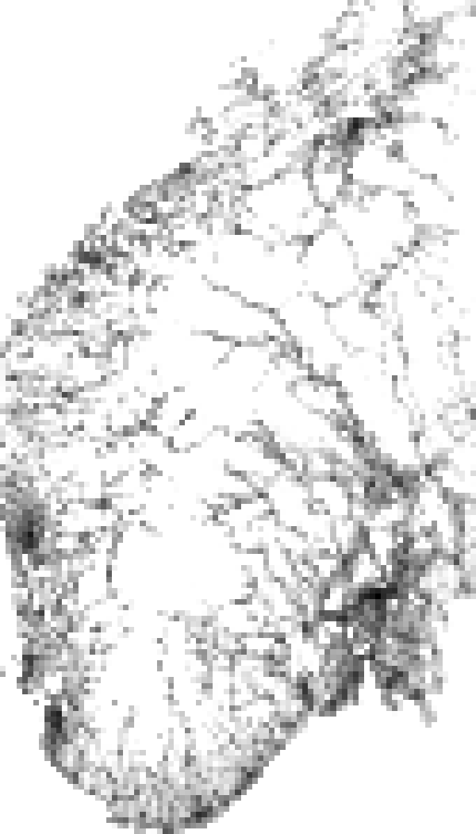
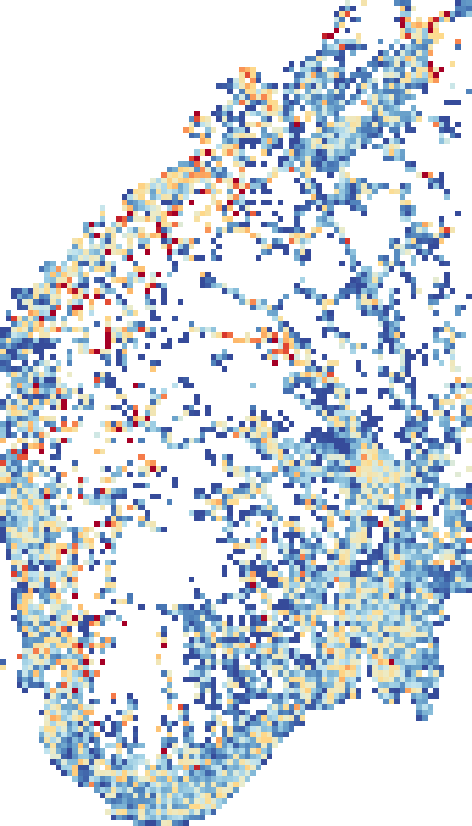
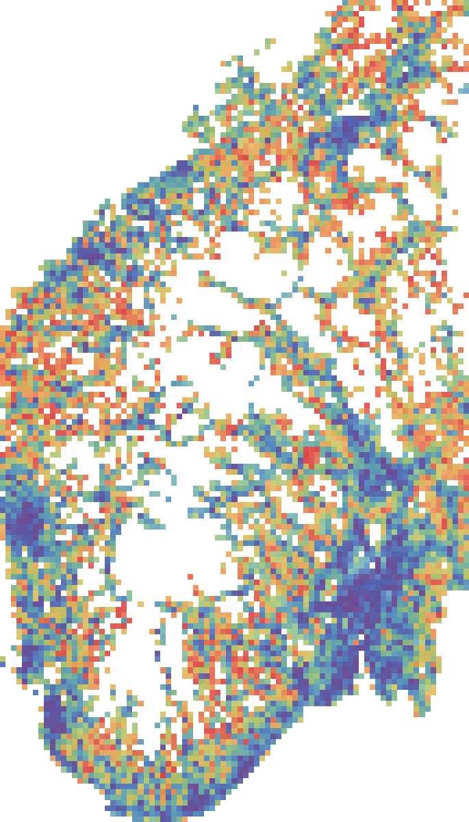
Gridded GDP → Neural Network
Gridded GDP estimates total GDP from each pixel
But it can systematically overpredict (blues) or underpredict (reds) true employment.
And has no information about sectoral composition.
An AI model can predict total employment and sectoral composition.
Context
Economic maps, locating which businesses operate where, are useful in many applications including:
- Constraining pollution sources / drivers of environmental impact
- Assessing vulnerability, e.g. to physical climate risk
- Performing regional economic impact assessments (disaster IO; building IRIOs)
The Knowledge Gap
A good map offers:
- Accessible without prohibitive costs
- Comprehensive covering more than fixed point sources
- Differentiates sectors, e.g. agriculture, industry, services
- Global, consistently covering many countries
The options available today are insufficient:
| Data Source | Accessible | Sector differentiation | Comprehensive coverage | Global coverage |
|---|---|---|---|---|
| National data | ✔️ | ✔️ | ✔️ | |
| Google Maps API | ✔️ | ✔️ | ✔️ | |
| Gridded GDP | ✔️ | ✔️ | ||
| Activity-specific data | ✔️ | ✔️ | ✔️ | |
| Predictive AI model? | ✅ | ✅ | ✅ | ✅ |
National data are rare, and not globally consistent. The Google Maps API is not accessible. Gridded GDP cannot differentiate sectors. Activity-specific data is not comprehensive.
Can a predictive AI model help?
Proposed Solution
Train an ML model to predict employment per sector in a map tile based on the surrounding features.
The Task: Learn how features (e.g. OpenStreetMap features, night luminosity, etc.) in a tile and surrounding neighborhood predict employment composition in a tile. Use training data from Norway on employment per sector in each tile.
Tile Example
Features
| Feature | # in tile |
|---|---|
| amenity=restaurant | 2 |
| amenity=school | 1 |
| building=residential | 10 |
| building=commercial | 3 |
| building=industrial | 0 |
| highway=primary (road) | 1 |
| highway=tertiary (road) | 4 |
| highway=path | 2 |
| landuse=industrial | 0 |
| landuse=residential | 1 |
| ... | ... |
| Total population | 500 |
Employment
| NACE section | Employees |
|---|---|
| A (Agriculture, forestry and fishing) | 0 |
| B (Mining and quarrying) | 0 |
| C (Manufacturing) | 33 |
| D (Electricity generation) | 3 |
| G (Wholesale and retail trade | 21 |
| H (Health care and social work) | 14 |
| ... | ... |
| Total employees | 71 |
Training data obtained from the Norwegian business register.
XGBoost Regression and Neural Network
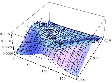
XGBoost builds a multivariate regression model. In this illustrative 3-dimensional graph, imagine the X axis is luminosity, the Y axis is # of buildings in the tile, and the Z axis is total employment. XGBoost builds a model from many input features to predict total employment in the tile.
Image source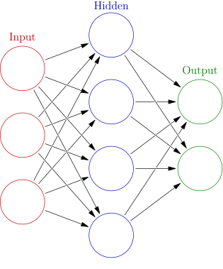
The neural network model accepts a vector of input features (e.g. # of schools, # of airports), and predicts a vector of output features (e.g. share of employment per sector).
Glosser.ca - Own work, Derivative of File:Artificial neural network.svg
Model Architecture
Steps:
- Filter out empty tiles to focus on inhabited areas
- Predict total employment per tile using an XGBoost regression model
- Predict employment composition (sector shares, summing to 1) per tile using a neural network
- Rescale to match national totals
For the prediction features currently we use OpenStreetMap and population. More features to explore, including: EO foundation model embeddings, building height data, and feature engineering to create derived features, e.g. distance to highways.
The model uses a wide spatial context window so predictions consider neighboring features (e.g. airports likely to have hotels nearby, etc.).
Training Data
Training data are from the Norwegian business register (processed & geocoded in ActMap).
1km grid data with employment per sector is also available for Japan. This data was withheld from training and used only for later validation.
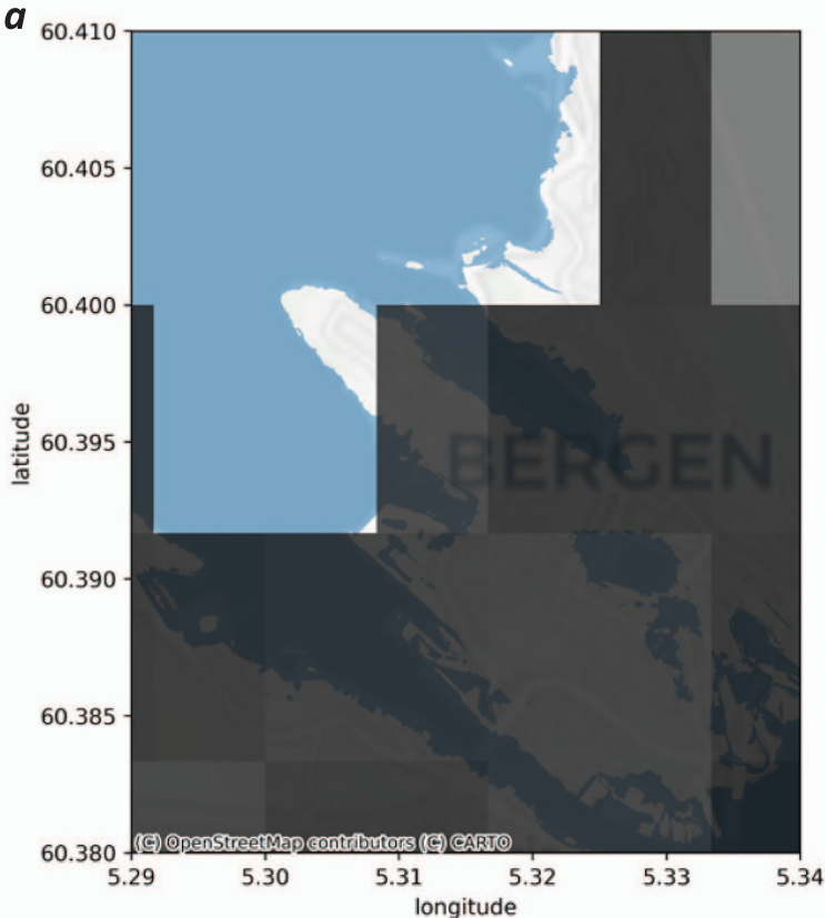
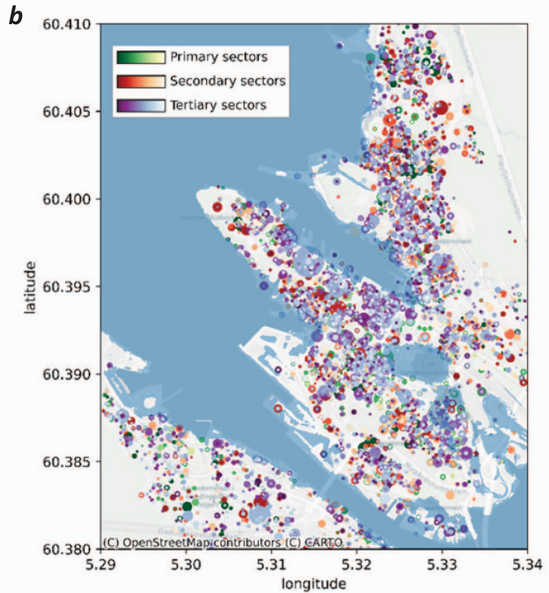
High resolution GDP modelling for climate risk assessments with an application to coastal flooding. Barre, F.I; Bouman, E.A.; Simpson, M.J.R.; Borck, H.S.; Hertwich, E.; Moran, D. 2025, Environ. Res. Lett. 20 094045 10.1088/1748-9326/adf867
How accurate is the model?
Step 1: Predict total employment per tile
Current state of the art: Using gridded GDP to estimate employment per tile:
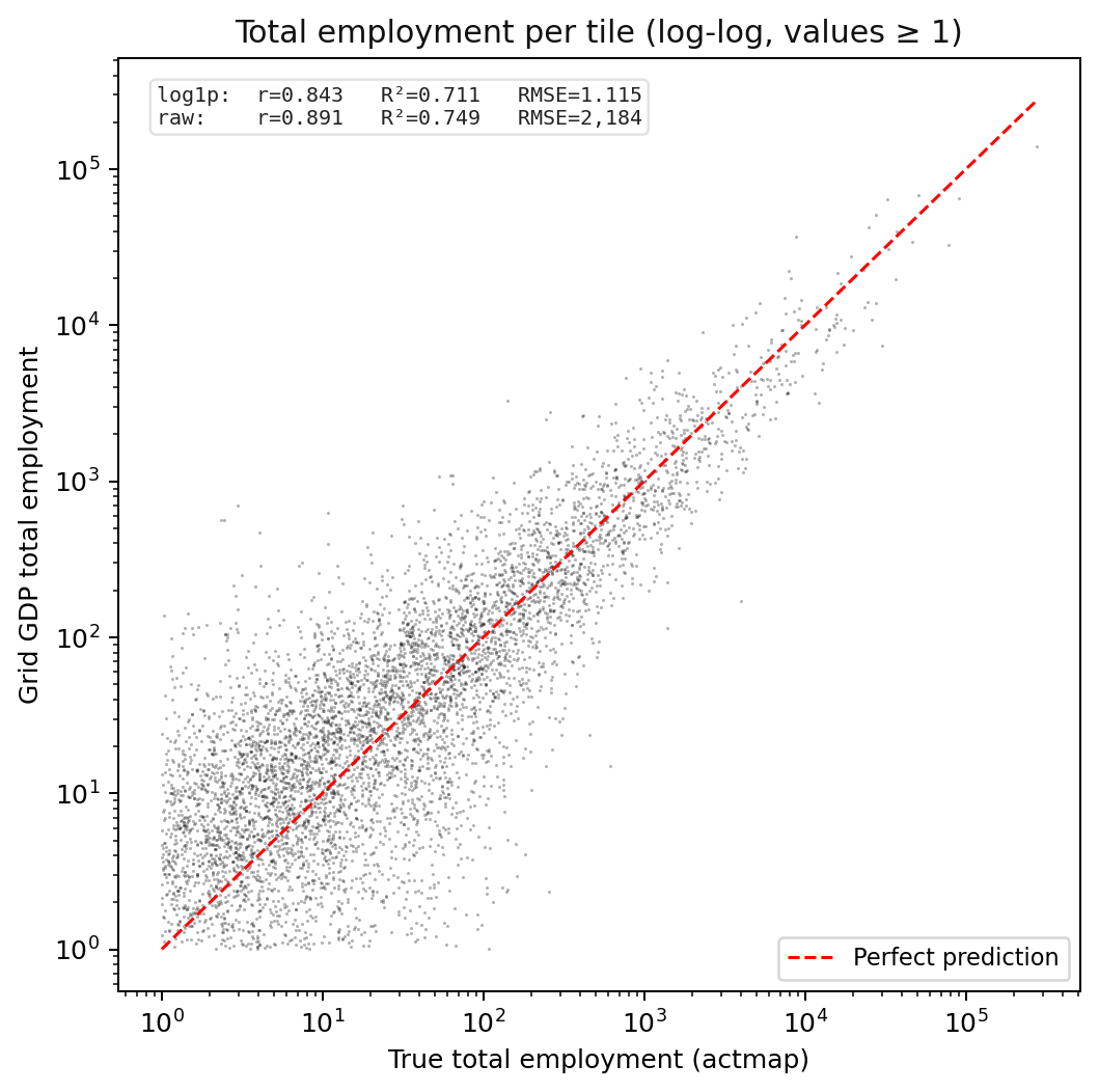
log1p R2 = 0.84.
Adding OSM features to better predict total employment, using XGBoost
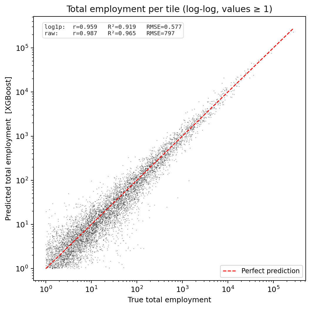
log1p R2 = 0.97.
How accurate is the model?
Step 2: Predict employment composition per tile
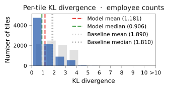
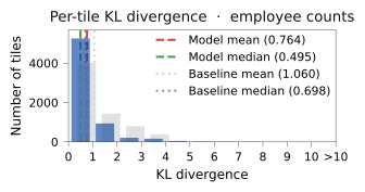
Kullback-Leibler divergence (KL) is a measure of how well the system predicts true employment composition for a tile. Low scores are better: a tile scores zero when the model can perfectly predict the true composition.
In this histogram we see the distribution of KL scores, comparing the gridded GDP approach (grey bars) to the model (blue bars).
The distribution of model KL scores (blue bars) closer to 0 indicates the model makes better predictions than the gridded GDP approach.
How accurate is the model?
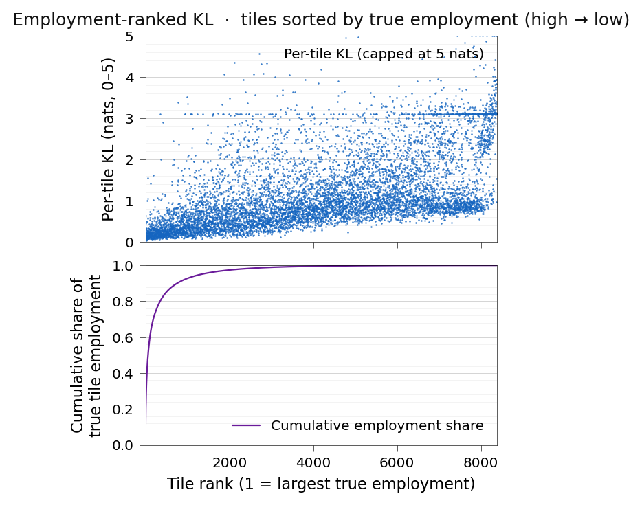
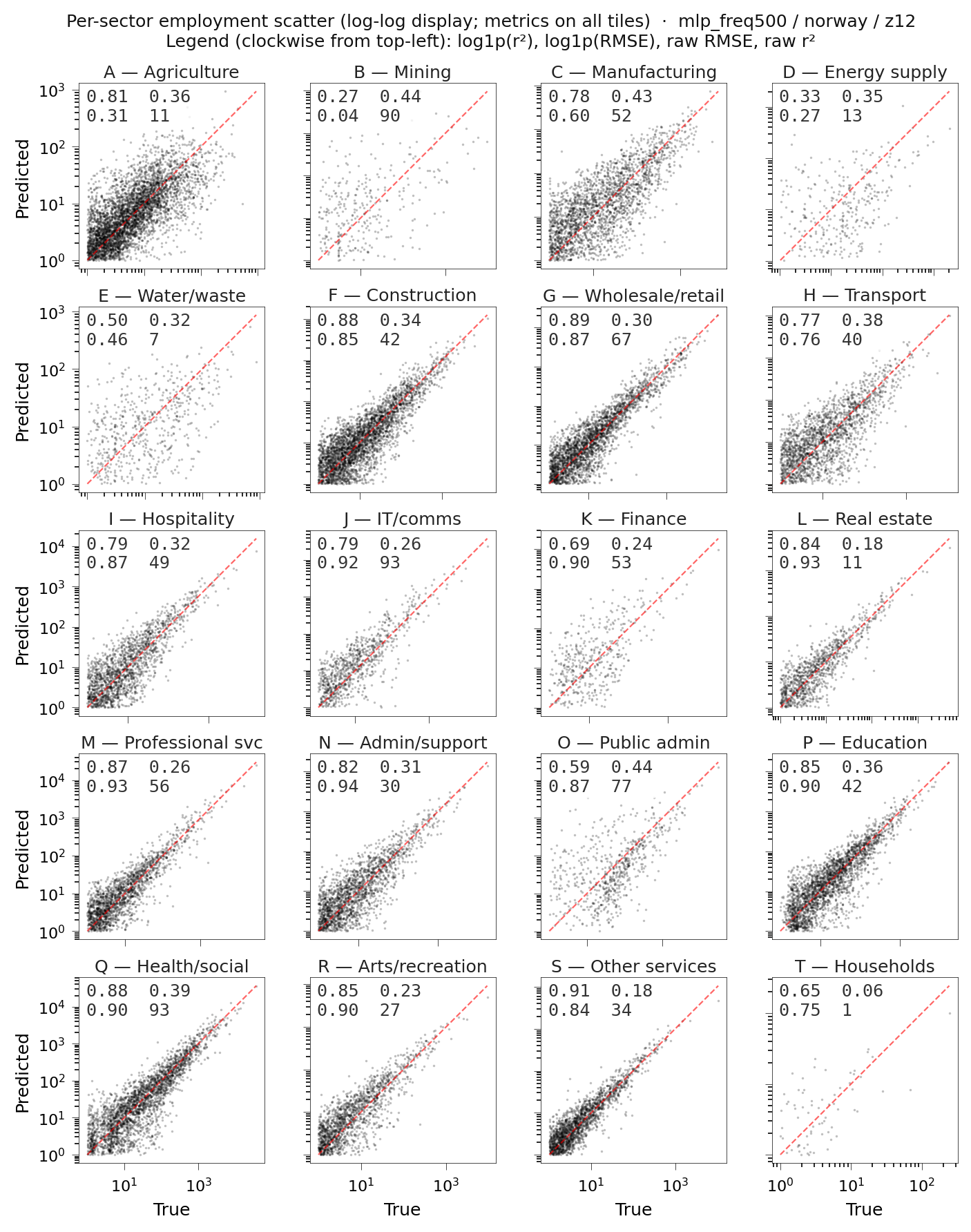
More important tiles are predicted more accurately.
Grid GDP predictive performance per sector, in Norway
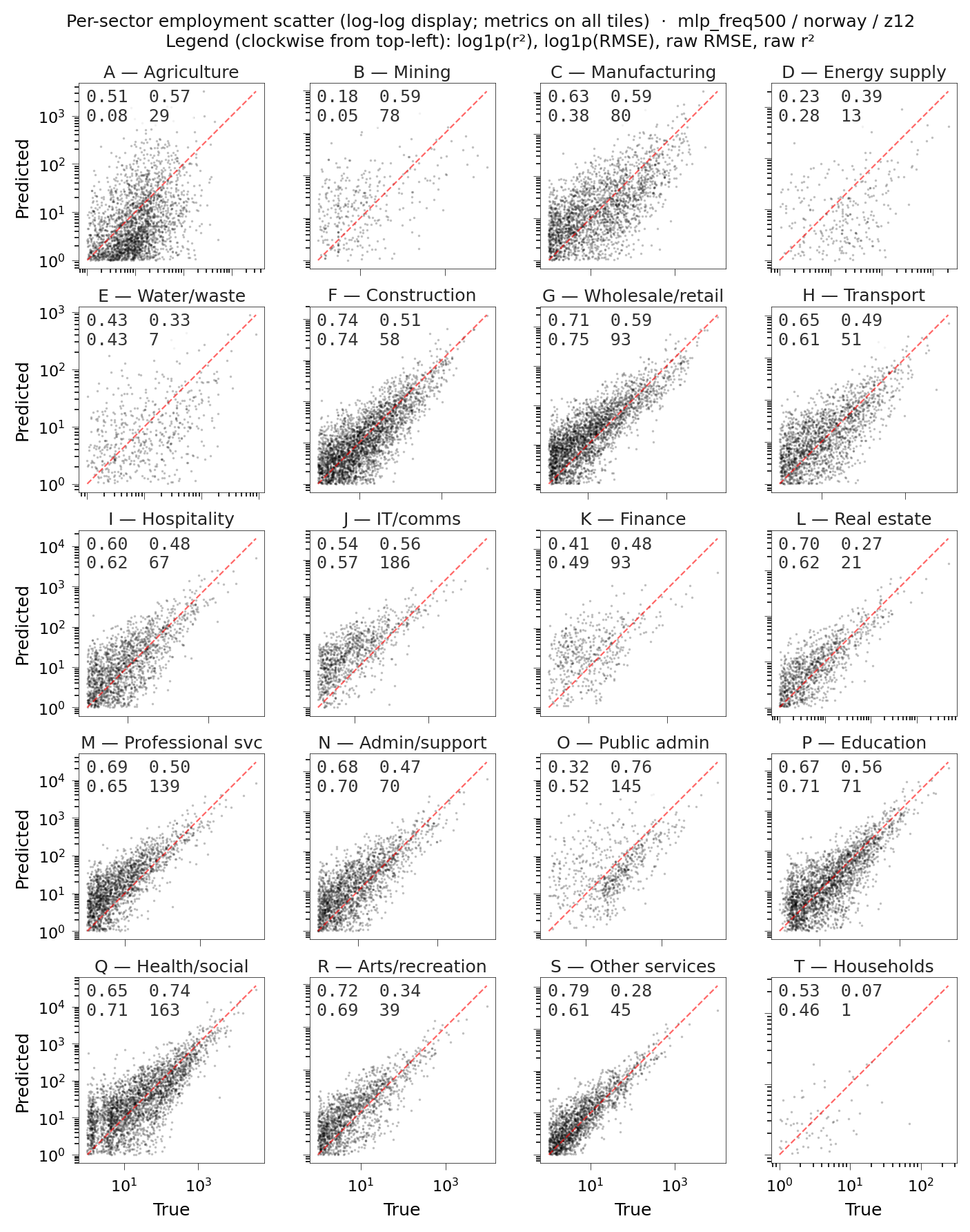
Model predictive performance per sector, in Norway
Transfer learning in Japan
Japan also provides employment per sector at 1km resolution. These were not used for training but can be used to evaluate transfer learning.
A leftward shift in KL scores is also seen for the predictions for Japan. This indicates the neural network has learned generalizable patterns.
A key limitation is the relatively small training dataset (~10,000 tiles). Using a finer grid mesh would not change the number of observations per variable, the crucial factor. More training data from other countries, even if only partial, will help.
Neural Network vs. Baseline
We can also see if the model predicts employment composition better than the gridded GDP approach commonly used today.
Left: improvement in log1p R2 over gridded GDP (larger is better).
Right: improvement in RMSE over gridded GDP (smaller is better).
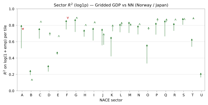
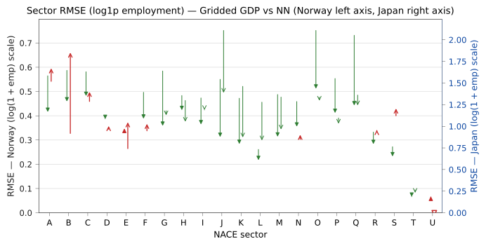
Filled arrows show data for Norway; hollow arrows show data for Japan.
Next Steps
- Paper preprint is published.
- Submission in process.
- Aim to scale regionally & globally
- Add feature and training data, improve core model
Recap
Goal: Estimate activity level (employment) per sector at high spatial resolution
Approach: Use machine learning to predict employment based on surrounding features
Training data: Norway public firm-level data
Tools: XGBoost regression and neural network
Results: Predictive performance is better than the baseline (gridded GDP)
Next steps: Scale it regionally & globally, make results available